Image Preprocessing and Augmentation
45 min readnotebookImage Fundamentals and Preprocessing
3 of 30Computer Vision with Deep Learning
Up next · Convolutional Neural Networks Explained
Train a flower classifier on photos taken on sunny afternoons and it will quietly learn that "bright" means "flower". Hand it a photo taken at dusk and watch the confidence collapse. The model did nothing wrong — it faithfully learned the dataset you gave it, sunshine and all. The problem is that your dataset was a narrow slice of the world, and the world will not hold still for your camera settings.
Two habits fix this, and they are the subject of this notebook. Preprocessing puts every input on a consistent scale — models don't eat raw pixels, they eat resized, normalized tensors, and the recipe must match exactly between training and serving. Augmentation attacks the narrow-slice problem head-on: it generates controlled variety — flips, crops, lighting shifts, noise — so the model rehearses the messiness of deployment while it still has labels to learn from. Together they are the cheapest accuracy you will ever buy: no new data, no bigger model, just discipline about what goes into the network. This notebook covers the full preprocessing pipeline and the augmentation patterns that matter most in practice.
pip install albumentations==1.4.21 torchvision==0.20.1 \
pillow==11.0.0 numpy==2.1.2torchvision.transforms.v2 for PyTorch-native
pipelines and albumentations for tasks where you also
need to transform bounding boxes or masks.
A trained model is a creature of habit: it expects inputs with exactly the statistics it saw during training, and it has no way to tell you when that expectation is violated. Preprocessing matters for three concrete reasons. Most architectures take a fixed input size (224 × 224 for ImageNet models, 384 × 384 for many ViTs), so arbitrary photos must be brought to that shape. Neural nets train better on values in roughly [-1, 1] than on raw [0, 255], so the numerical range must be rescaled. And because the model memorizes the statistics of whatever it was fed, preprocessing at training and at inference must be identical, or you ship garbage.
In practice these three requirements collapse into a short recipe that has barely changed in a decade. Here it is, in the form you will type hundreds of times:
import torch
from torchvision.transforms import v2 as T

train_tx = T.Compose([
    T.RandomResizedCrop(224, scale=(0.7, 1.0), antialias=True),
    T.RandomHorizontalFlip(p=0.5),
    T.ColorJitter(brightness=0.2, contrast=0.2, saturation=0.2, hue=0.02),
    T.ToImage(),                            # PIL/ndarray → (C, H, W) tensor
    T.ToDtype(torch.float32, scale=True),   # uint8 [0, 255] → float32 [0, 1]
    T.Normalize(mean=[0.485, 0.456, 0.406],   # ImageNet stats
                std =[0.229, 0.224, 0.225]),
])

eval_tx = T.Compose([
    T.Resize(256, antialias=True),
    T.CenterCrop(224),
    T.ToImage(),
    T.ToDtype(torch.float32, scale=True),
    T.Normalize(mean=[0.485, 0.456, 0.406],
                std =[0.229, 0.224, 0.225]),
])
This is torchvision.transforms.v2 — the current
default, and what you should reach for in new code. It is faster
than the legacy API, works on tensors and PIL images alike, and
(as you will see in Section 8) can transform bounding boxes and
masks in lockstep with the image. The explicit
ToImage + ToDtype pair replaces the old
ToTensor, separating "make it a tensor" from "make it
float in [0, 1]" so nothing happens by magic.
Two pipelines: training augments aggressively; evaluation is
deterministic. The split is non-negotiable — augmenting at eval
time produces non-reproducible numbers. Notice that both end with
the same Normalize call, and that its two triplets of
constants look suspiciously specific. They are.
What does normalization actually do? Subtracting the mean recenters each channel around zero; dividing by the standard deviation puts all three channels on the same scale. In words: "make the input look statistically like every input the network has ever seen". Gradients behave better on centered data, and pretrained weights are calibrated to it.
T.ColorJitter(brightness=0.4, contrast=0.4, saturation=0.4, hue=0.1)
T.RandomGrayscale(p=0.1)
T.GaussianBlur(kernel_size=3, sigma=(0.1, 2.0))
Color jitter handles lighting variation. Grayscale (low p) helps the model not rely on color when it shouldn't. Blur simulates out-of-focus shots. The right intensity is task-dependent — a medical-imaging classifier should not have its hue rotated by 0.5.

Library calls can make augmentation feel like magic, so it is
worth seeing how little is actually happening. The cell below
builds a synthetic 64 × 64 image and applies four classic
augmentations — horizontal flip, crop-and-downsample, brightness
scaling, gaussian noise — using nothing but numpy indexing and
arithmetic. It also normalizes the image and prints the statistics
before and after, so you can watch the mean move to 0 and the
standard deviation to 1. Press Run, then change
which augmentation is displayed (swap noisy for
flipped, cropped, or bright)
and run again.
Notice what the printed stats tell you: the augmented copies keep the bright object recognizably in place — a model would still call it the same label — while normalization changes the numbers completely without changing the picture at all. That is the division of labor: augmentation varies what the model sees, normalization standardizes how it is delivered. The classics above cover most projects; modern training recipes push further.
Hand-picking augmentations and their strengths is fiddly, so the field automated it. Two families dominate modern training recipes: policy augmentations, which randomly sample transforms from a fixed menu, and mixing augmentations, which combine two labeled images into one training example.
| Augmentation | What it does | Helps when |
|---|---|---|
| RandAugment | Applies N random transforms at magnitude M (two knobs) | The classic strong-recipe default |
| TrivialAugment | One random transform, random magnitude — zero knobs | Matches RandAugment with nothing to tune; a great modern default |
| AugMix | Mixes augmented chains; strong robustness | You care about distribution shift |
| Cutout / Random Erasing | Masks a random rectangle | Fights overfitting on small data |
| MixUp | Blends two images pixel-wise, blends their labels the same way | Strong regularization, low-data regime |
| CutMix | Pastes a patch of one image into another, splits the label by area | Object-centric classification |
train_tx = T.Compose([
    T.RandomResizedCrop(224, antialias=True),
    T.RandomHorizontalFlip(),
    T.TrivialAugmentWide(),                 # or T.RandAugment(num_ops=2, magnitude=9)
    T.ToImage(),
    T.ToDtype(torch.float32, scale=True),
    T.Normalize([0.485, 0.456, 0.406], [0.229, 0.224, 0.225]),
    T.RandomErasing(p=0.25),
])
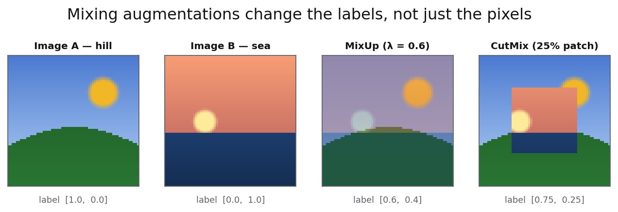
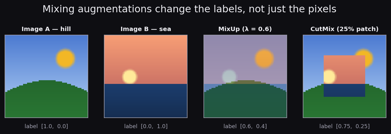
The mixing augmentations are stranger — and worth a picture. MixUp
takes two images and computes lam * img_a + (1 - lam) * img_b;
a 60/40 blend of a dog and a plane is a ghostly double exposure no
photographer would produce, yet training on it regularizes the
model beautifully. CutMix pastes a rectangular patch instead. The
crucial detail in both: the label changes too.
# MixUp / CutMix operate on BATCHES, so they live in the collate_fn,
# not in the per-image transform:
cutmix = T.CutMix(num_classes=1000)
mixup  = T.MixUp(num_classes=1000)
mix    = T.RandomChoice([cutmix, mixup])

def collate_fn(batch):
    return mix(*torch.utils.data.default_collate(batch))

loader = DataLoader(dataset, batch_size=64, collate_fn=collate_fn)
Everything so far transforms an image alone. The moment your task has labels with spatial coordinates — bounding boxes, masks, keypoints — a flipped image with un-flipped boxes is worse than no augmentation at all, and you need a tool that moves both together.
Two tools do this well. Albumentations is the community standard for detection and segmentation work: it augments images and their associated bounding boxes, masks, and keypoints — together, consistently — with a large menu of transforms and very fast OpenCV-backed implementations.
import albumentations as A

train_tx = A.Compose([
    A.RandomResizedCrop(size=(224, 224), scale=(0.7, 1.0)),
    A.HorizontalFlip(p=0.5),
    A.ColorJitter(0.2, 0.2, 0.2, 0.02, p=0.8),
    A.Normalize(mean=(0.485, 0.456, 0.406), std=(0.229, 0.224, 0.225)),
], bbox_params=A.BboxParams(format="yolo", label_fields=["class_ids"]))

out = train_tx(image=img, bboxes=boxes, class_ids=ids)
img_aug, boxes_aug = out["image"], out["bboxes"]
The PyTorch-native alternative: torchvision.transforms.v2
understands tv_tensors.BoundingBoxes and
tv_tensors.Mask wrappers, and every geometric
transform in the v2 pipeline moves them along with the image
automatically. If your project already lives in torchvision, v2
keeps everything in one library; if you want the widest transform
menu and maximum speed, Albumentations remains the pick. Either
way, never transform image and labels through separate code
paths.
Here is the frame that makes every augmentation decision easier. Each transform you enable is a claim about your problem: "the label is invariant to this change". Horizontal flip claims left-right doesn't matter; color jitter claims exact hue doesn't matter; a crop claims the label survives losing the edges. When the claim is true, you have injected free prior knowledge — the model no longer wastes capacity learning that lighting is irrelevant, which is exactly what a regularizer does. Like any regularizer, dose it by the overfitting gap: a big model on small data wants strong augmentation and long training; a small model that is already underfitting wants less.
And when the claim is false, augmentation manufactures mislabeled data at scale. The classic cases:
The test is always the same: apply the transform, then ask a domain expert to label the result. If their answer changes — or they refuse to answer — the augmentation is off the menu.
Augmentation is one of the few tools in deep learning that can actively hurt you when applied thoughtlessly, and the failure modes are predictable enough to list. Read these now; you will meet each of them eventually:
timm.data.resolve_model_data_config(model) returns
the exact mean, std, input size, and interpolation to use.
With scaling settled, the next question is geometry — how a photo of arbitrary size becomes exactly 224 × 224.
| Operation | What it does | When to use |
|---|---|---|
Resize(N) | Scale shorter side to N, preserve aspect | Keep all content, fixed size for next step |
CenterCrop(N) | Take central N × N square | Eval-time deterministic crop |
RandomResizedCrop(N) | Random box, resized to N × N | Training augmentation |
Pad(p) | Add border | Preserve content without distortion |
Resize + Pad ("letterbox") | Scale then pad to a fixed shape | Detection (preserve aspect for boxes) |
Resizing looks trivial and hides three real bugs. First,
aspect ratio: Resize((224, 224))
with a tuple stretches a 3:4 photo into a square — every object
gets 33% wider, and a detector trained this way learns deformed
geometry. Use scalar Resize(224) (shorter side) plus
a crop, or letterbox padding for detection. Second,
interpolation: bilinear is the safe default for
photos; bicubic is what many ViT recipes expect (another thing the
timm data config tells you); and nearest is mandatory for
segmentation masks — bilinearly interpolating class IDs invents
classes that don't exist, like "half road, half sky" averaging to
"car". Third, antialiasing: when downscaling
tensors, pass antialias=True so high-frequency detail
is filtered out instead of aliasing into noise — PIL always
antialiases, tensors historically didn't, and models trained on
one and served on the other quietly lose accuracy.
Resizing makes inputs legal; augmentation makes models robust. The idea is almost embarrassingly simple: if you want the model to survive flipped, shifted, oddly-cropped photos in production, show it flipped, shifted, oddly-cropped photos in training. Each transformed copy keeps its label, so one annotated image does the work of many.
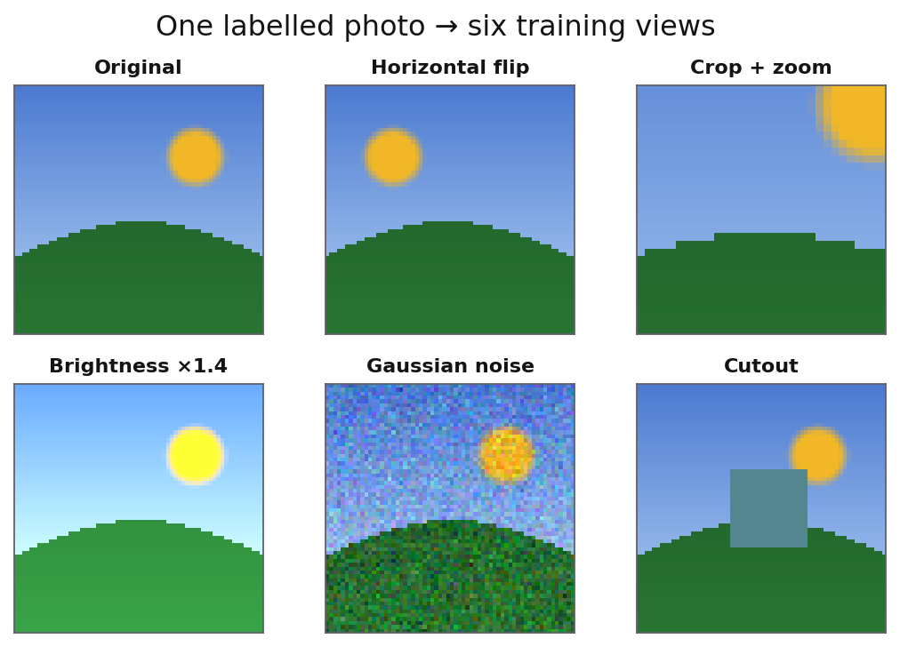
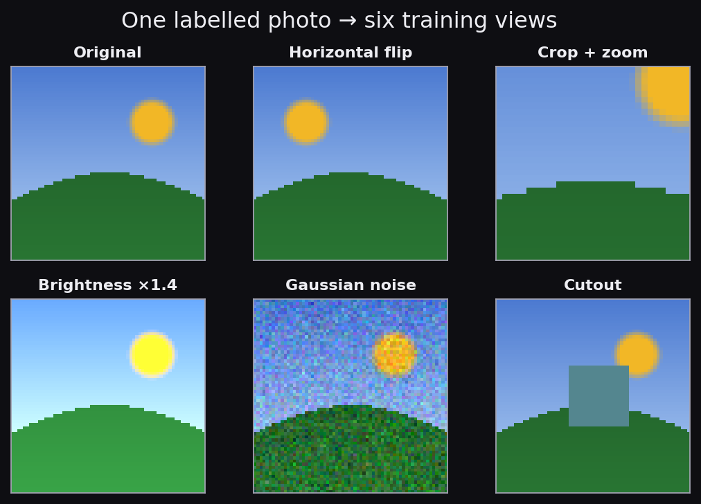
The geometric classics apply to almost every task. Horizontal flip doubles your effective data for free on most natural images, though you should skip it for digits, text, and scenes where left and right carry meaning, such as road signs. Small random rotations, roughly -15° to +15°, cover the tilt of a handheld camera; larger angles rarely help unless your data genuinely contains them. Random crops and scale changes handle variation in position and size, and a random affine transform bundles translation, rotation, and scale into a single one-stop augmentation. Perspective warps earn their keep when test-time camera angles differ from training, as they do for documents and signs photographed from odd positions.
Geometry covers where things are; color augmentations cover how the light was — the difference between the sunny-afternoon training set and the dusk photo that broke it:
antialias=True on
tensor downscales quietly costs accuracy; eval with a
different interpolation than the checkpoint expects does
too.You can now take any pile of images and turn it into what a network actually wants: consistently sized, correctly normalized tensors, with training-time variety that rehearses the conditions of deployment — and you know the handful of ways this goes wrong. What you don't yet know is what happens on the other side of the tensor. Lesson 4 opens the box: the convolutional neural network, the architecture that consumes every batch you just learned to prepare.