Image Representation and Color Spaces
40 min readnotebookImage Fundamentals and Preprocessing
2 of 30Computer Vision with Deep Learning
Up next · Image Preprocessing and Augmentation
Here is a debugging story you will live through at least once. A team trains a classifier that reaches 94% accuracy in the notebook, ships it, and watches it label photographs of golden retrievers as "traffic light". Nothing is wrong with the model. The serving code simply loads images with a different library than the training code did — and the two libraries disagree about the order of color channels. The model learned on RGB and is being fed BGR: every red pixel arrives as blue, and features that took days to train now fire on the wrong things. No exception is raised. Nothing crashes. The predictions are just quietly, completely wrong.
Bugs like this are why this lesson exists. Before you train any model, you need to understand what an image is to a computer: an array of integers organized as height × width × channels, wrapped in conventions — channel order, value range, memory layout — that differ between libraries and fail silently when mixed. This notebook walks through pixels, channels, color spaces, and the small library of operations (read, resize, convert, normalize) that every vision pipeline relies on. None of it is glamorous; all of it will save you hours of the kind of debugging that starts with "but it worked yesterday".
pip install pillow==11.0.0 numpy==2.1.2 opencv-python==4.10.0.84 \
matplotlib==3.9.2 torch==2.5.1 torchvision==0.20.1torchvision.datasets.FakeData
works if you have nothing else handy.
Start with the one fact everything else builds on. Open any photograph in Python and what you get back is not a picture — it is a rectangular block of numbers:
from PIL import Image
import numpy as np

img = Image.open("cat.jpg")             # PIL Image, 'RGB' mode
arr = np.array(img)
print(arr.shape, arr.dtype)             # (H, W, 3), uint8
print(arr.min(), arr.max())             # 0, 255
Three facts about that block are worth committing to memory before anything else. In numpy the shape is (H, W, C), height first, which surprises people who think in "width × height". The dtype is almost always uint8, so values run from 0 to 255. And the channels come last in numpy and PIL, whereas PyTorch puts them first, as (C, H, W). Mixing up (H, W, C) and (C, H, W) is the single most common cause of "this code ran yesterday and now it crashes" in vision pipelines. Now that you know the container, consider what the three channels actually mean.
Each pixel holds three numbers because your screen mixes three
primaries. A pixel of [255, 0, 0] is pure red;
[255, 255, 255] is white; [30, 30, 30]
is a dark gray. A full-color image is therefore three stacked
grayscale images — one measuring "how red", one "how green", one
"how blue" at every location:
# RGB: 3 channels, ordered red-green-blue (PIL convention)
print(arr[0, 0])                        # [R, G, B] for the top-left pixel

# Grayscale: 1 channel
gray = img.convert("L")                 # PIL "luminance"
print(np.array(gray).shape)             # (H, W)
Grayscale is computed as a weighted sum
(0.299·R + 0.587·G + 0.114·B) approximating human
perception of brightness. Read the formula in words: green
contributes almost 60% of perceived brightness, red about 30%, and
blue barely 11%. The weights are not arbitrary — human retinas
carry far more green-sensitive cones than blue ones, so a naive
equal-weight average would look wrong to us. The formula
is essentially a small model of
your own eye. Many CV operations (edge detection, classical
features) traditionally happened in grayscale; deep models almost
always use the full 3 channels.
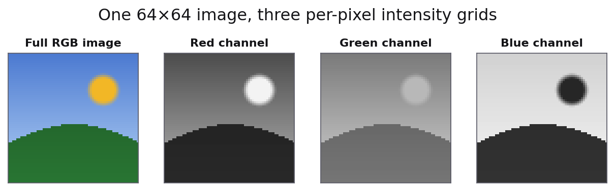
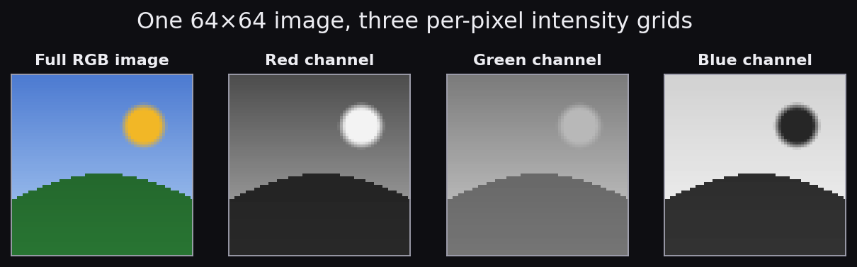
Reading about channels is one thing; building an image out of them is better. The cell below constructs a 64 × 64 RGB image from raw numpy — a red gradient running left to right, a blue gradient top to bottom, plus a red square and a green disk — then splits out the red channel and converts one pixel to grayscale by hand. Press Run and check the printed shapes against the (H, W, C) convention; then look at the right panel and notice that the "red channel" is itself just a grayscale intensity map.
Two details worth noticing in the output. The red square scores hot in the red channel but its grayscale value is only about 0.37 — red contributes little to brightness. The green disk, at a similar overall intensity, lands near 0.58 because green dominates the luminance formula. RGB is only the most common way to carve up color, though — and the alternatives exist because different jobs need different carvings.

A color space is a coordinate system for color, and like map projections, each one distorts something to make something else convenient. HSV separates what color (hue) from how much light (value), which makes "find everything orange" a one-line threshold instead of a three-channel puzzle. Lab is engineered so that equal distances feel equally different to a human. You will spend 95% of your time in RGB, but knowing when to switch is a quiet superpower:
| Space | Channels | When you'd use it |
|---|---|---|
| RGB | R, G, B | Default; what every model expects |
| BGR | B, G, R | OpenCV's default — silently wrong color when displayed as RGB |
| HSV | Hue, Saturation, Value | Color-based filtering, augmentations like "shift hue" |
| Lab | Lightness, a*, b* | Perceptually uniform; image-similarity metrics |
| YCbCr | Luminance + chroma | JPEG compression, video codecs |
Two rows deserve their backstory. YCbCr exists because your eye is far sharper about brightness than about color: JPEG and virtually every video codec convert to YCbCr and store the two chroma channels at half resolution (the "4:2:0" you see in codec specs), throwing away color detail you would never miss. Every JPEG you have ever loaded made a round trip through this space. Lab is built so that the numeric distance between two colors approximates how different they look — which is why print shops and quality-control systems measure color error in Lab (as "delta E"), and why some augmentation and color-transfer tricks operate there.
import cv2
bgr = cv2.imread("cat.jpg")             # OpenCV reads as BGR!
rgb = cv2.cvtColor(bgr, cv2.COLOR_BGR2RGB)
hsv = cv2.cvtColor(rgb, cv2.COLOR_RGB2HSV)
lab = cv2.cvtColor(rgb, cv2.COLOR_RGB2LAB)
Remember that the opening bug of this lesson produced no error message. Range mismatches are the same species of silent failure: a model trained on values in [0, 1] that receives values in [0, 255] doesn't crash — it just outputs noise with confidence. Four dtypes cover nearly everything you will meet:
| dtype | Range | Where you meet it |
|---|---|---|
| uint8 | 0 … 255 | JPEG, PNG, everything on disk and on screens |
| uint16 | 0 … 65 535 | Medical DICOM (typically 12-16 bits used), RAW camera files, microscopy |
| float32 | usually [0, 1] or normalized | What models consume; the default compute dtype |
| float16 / bfloat16 | as float32 | Mixed-precision training and inference; half the memory |
img_f = arr.astype(np.float32) / 255.0
print(img_f.min(), img_f.max())         # 0.0, 1.0
Bit depth tells you how finely intensities are quantized. But it says nothing about which physical brightness each number represents — and that mapping hides one more convention worth knowing about.
The pixel values in an ordinary image are not proportional to physical light. They are gamma-encoded: the sRGB standard applies a curve (roughly a power of 1/2.2) that spends more of the 256 available codes on dark tones, where human eyes are most discriminating, and fewer on highlights. A pixel of 128 is therefore not "half as bright" as 255 — physically it is closer to a fifth as bright.
For deep learning you can mostly ignore this: models train and infer on gamma-encoded values, and as long as training and serving agree, the network never notices. For classical image processing it occasionally bites. Strictly correct resizing, blurring, and blending should happen in linear light (decode the gamma, operate, re-encode), and standard pipelines skip this step, which is why naive downscaling can darken fine bright detail. Know the issue exists so you recognize it when a physicist or a graphics engineer brings it up. HDR formats (10-bit HDR10, camera RAW, OpenEXR floats) store a wider brightness range with different transfer curves, but vision pipelines almost always tone-map HDR down to standard 8-bit sRGB before the model ever sees it.
Ranges and curves answer "what values live in each cell"; the next convention answers "in what order are the cells arranged" — and it is the one where numpy and PyTorch part ways.
import torch
# numpy / PIL: (H, W, C)
print(arr.shape)                        # (224, 224, 3)
# PyTorch:    (C, H, W)
ten = torch.from_numpy(arr).permute(2, 0, 1)
print(ten.shape)                        # (3, 224, 224)

# The modern torchvision v2 conversion — explicit about layout and scaling:
from torchvision.transforms import v2 as T
tensor = T.Compose([
    T.ToImage(),                        # PIL/ndarray → CHW tensor
    T.ToDtype(torch.float32, scale=True),  # uint8 [0,255] → float32 [0,1]
])(img)
Why two conventions? PyTorch's choice (C, H, W) makes batched data
shape (N, C, H, W), which is friendlier to convolutions because
the spatial dimensions stay together. NumPy and PIL chose (H, W, C)
because that's how image data is stored on disk. Train yourself to
read shape tuples carefully. One footnote for later: on modern
GPUs, PyTorch can store an NCHW tensor with channels-last
memory layout (x.to(memory_format=torch.channels_last))
for faster convolutions — the logical shape you index stays NCHW,
only the bytes are rearranged. File it away for the performance
lessons.
With the in-memory conventions settled, the remaining mechanics are getting pixels on and off disk:
from PIL import Image

# Read
img = Image.open("input.jpg")           # lazy; data not loaded yet
img.load()                              # force load

# Write
img.save("output.png")                  # PNG (lossless)
img.save("output.jpg", quality=92)      # JPEG with quality

# Straight to a tensor, skipping PIL entirely:
from torchvision.io import decode_image
ten = decode_image("input.jpg")         # uint8 tensor, (C, H, W), RGB
PIL is the cleanest API for I/O; torchvision's
decode_image returns a CHW tensor directly and keeps
the whole pipeline in PyTorch; OpenCV is fastest for video. Pick
by need: PIL for clarity, torchvision for PyTorch pipelines,
OpenCV for high-throughput frame processing.
Looking at your data is the cheapest debugging tool in vision — most of the silent failures in this lesson are instantly visible the moment you plot a batch. Make it a reflex:
import matplotlib.pyplot as plt

fig, ax = plt.subplots(1, 3, figsize=(12, 4))
ax[0].imshow(arr); ax[0].set_title("RGB")
ax[1].imshow(np.array(gray), cmap="gray"); ax[1].set_title("Gray")
ax[2].imshow(arr[..., 0], cmap="gray"); ax[2].set_title("R channel")
for a in ax: a.axis("off")
plt.show()
Single-channel data needs cmap="gray"; otherwise
matplotlib applies the default viridis colormap and your image
looks alien. Triple-check colormaps in any vision plot you commit.
Because an image is an array, every spatial operation you can name is an indexing expression in disguise. No special libraries, no loops — just coordinates:
# Top-left 100×100 patch
patch = arr[:100, :100]

# Center crop
H, W = arr.shape[:2]; s = 224
top  = (H - s) // 2; left = (W - s) // 2
center = arr[top:top + s, left:left + s]

# Mask: where red is dominant
mask = (arr[..., 0] > 150) & (arr[..., 0] > arr[..., 1] + 30)
print(mask.shape, mask.dtype)           # (H, W), bool
Numpy slicing is the universal language of vision preprocessing.
Crops, masks, color-thresholding, channel splits — all of them
reduce to a few lines of arr[...]. Lesson 3 will
build entire augmentation pipelines out of exactly these
primitives. Before you get there, one habit is worth installing
permanently.
You now hold every convention this lesson has introduced. Here is the complete journey of one image through a modern PyTorch pipeline, with the shape, dtype, and range annotated at every step — this is the mental x-ray you should be able to produce for any pipeline you ever touch:
import torch
from torchvision.io import decode_image
from torchvision.transforms import v2 as T

x = decode_image("cat.jpg")             # (3, H, W)   uint8    [0, 255]  RGB

pipeline = T.Compose([
    T.Resize(256),                      # (3, 256, W') uint8   [0, 255]
    T.CenterCrop(224),                  # (3, 224, 224) uint8  [0, 255]
    T.ToDtype(torch.float32, scale=True),  # float32 [0, 1]
    T.Normalize(mean=[0.485, 0.456, 0.406],
                std =[0.229, 0.224, 0.225]),  # float32, per-channel ~N(0, 1)
])

x = pipeline(x)                         # (3, 224, 224) float32, mean ≈ 0
batch = x.unsqueeze(0)                  # (1, 3, 224, 224) — models want NCHW
logits = model(batch)                   # (1, num_classes) float32
You can now do what the unlucky team in the opening story could not: look at any image tensor and interrogate it — shape, dtype, range, channel order — before it ever reaches a model. That discipline turns silent failures into thirty-second fixes. Next, Lesson 3 puts these primitives to work: resizing, normalizing, and augmenting images into the tensors a network actually trains on.