Introduction to Computer Vision

Introduction to Computer Vision

Computer vision teaches machines to see — to take an array of pixel values and extract meaning: a face, a tumour, a stop sign, a defect on a circuit board. The field went from "researchers can recognize handwritten digits" to "self-driving cars and medical imaging diagnostics" in roughly a decade, driven almost entirely by deep learning. This lesson sets the map for the next 29 — what computer vision is, why it works now, and where it is going.

1. What Computer Vision Actually Does

At its core, every computer-vision task takes an image (or video) and produces structured output. The five canonical tasks:

Task	Output	Example
Classification	One label per image	"cat" / "dog"
Detection	Boxes + labels	"person at (x, y, w, h)"
Segmentation	Pixel-wise label map	"this pixel is road, this is sky"
Generation	A new image	"a photo of an astronaut on a horse"
Multi-modal	Text + image jointly	"describe this picture"

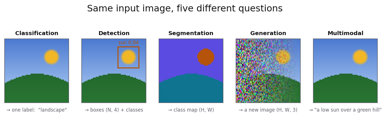
The course covers all five. Sections 1-2 build classification; Section 3 adds detection; Section 4 adds segmentation; Section 5 generation; Section 6 the modern multi-modal landscape.

2. Why Vision Is Hard (For Machines)

Humans recognize a cat from any angle, in any lighting, behind any occlusion. A computer sees a 224 × 224 × 3 array of integers from 0 to 255. The challenge is the gap between those numbers and "cat".

• Viewpoint variation — same cat, different angles → very different pixel arrays.
• Illumination — sunlit cat vs night cat.
• Scale — close-up cat vs distant cat.
• Occlusion — only the tail is visible.
• Background clutter — cat in a busy room.
• Intra-class variation — Persian, Maine Coon, Sphynx are all "cats" but look very different.

Pre-deep-learning systems handled these with hand-engineered features (SIFT, HOG, SURF). Deep nets learn the right features directly from data — that one shift is what unlocked the modern era.

3. The Pre-Deep-Learning Era (Briefly)

Before 2012, computer vision was a pipeline of:

1. Hand-designed feature extractors (SIFT, HOG, SURF).
2. A classical classifier (SVM, random forest) on top.
3. Domain-specific tricks per task.

Performance plateaued in the high 70s % on ImageNet classification. Each new task required new features. It was research-heavy, brittle, and didn't generalize.

4. The 2012 Inflection Point

Within five years, ImageNet classification went from "human performance is the goal" to "humans are the bottleneck". By 2017, top models were beating the human baseline. The same architectural ideas powered detection, segmentation, and eventually generation.

5. Why Deep Learning Wins for Vision

Three properties of vision data that deep learning exploits:

• Local structure — nearby pixels are highly correlated. Convolutions exploit this directly.
• Translation invariance — a cat is a cat whether it's in the top-left or bottom-right. Convolutions share weights across spatial positions.
• Hierarchy — pixels → edges → textures → parts → objects. Stacking convolutional layers builds the same hierarchy automatically.

CNNs (Lesson 4) are the architecture that bakes these three inductive biases into the model. Sections 1-4 use CNNs heavily; Section 5-6 introduce Transformers, which trade some of these biases for flexibility.

6. The Modern Vision Stack

Layer	What it provides
Frameworks	PyTorch, TensorFlow / Keras
Vision libraries	torchvision, timm (1000+ pretrained models)
Image I/O	Pillow (PIL), OpenCV
Augmentation	Albumentations, torchvision.transforms.v2
Detection / segmentation	Ultralytics (YOLO), detectron2, MMDetection
Generation	diffusers, Stable Diffusion, ComfyUI
Multi-modal	CLIP, BLIP, LLaVA, transformers

This course uses PyTorch + torchvision as the primary stack, introduces timm in Section 2, switches to Ultralytics for detection in Section 3, and uses 🤗 diffusers for Section 5.

7. Where Computer Vision Is Used Today

• Healthcare — diabetic retinopathy screening, tumor detection in MRI/CT, dermatology classification.
• Autonomous vehicles — perception for lane keeping, pedestrian detection, traffic-light classification.
• Manufacturing — defect detection on assembly lines; reads QR codes and serial numbers reliably.
• Retail — Amazon Go-style checkout-free stores; shelf-monitoring; product recognition.
• Agriculture — drone imagery for crop health, pest detection, yield prediction.
• Content moderation — flagging harmful images and videos at scale.
• Creative tools — Photoshop's generative fill, DALL·E, Midjourney, Stable Diffusion.

8. The Cost: Data and Compute

Deep vision works because of two kinds of scale:

• Data — ImageNet has 1.2 M labeled images across 1000 classes. Modern pretraining datasets (LAION, JFT) have billions.
• Compute — training a state-of-the-art model from scratch costs thousands to millions of GPU-hours.

Practical implication: most real-world projects don't train from scratch. Transfer learning (Lesson 7) starts from a pretrained model and fine-tunes — accuracy that would have taken months and millions in 2012 now takes minutes and a single GPU.

9. What This Course Will Build

10. The Road Ahead

Computer vision in 2026 is moving toward three frontiers:

1. Foundation models — one model handling many vision tasks (SAM for segmentation, DINOv2 for features, CLIP for embeddings).
2. Multi-modal — vision + language jointly, enabling "describe this image", "find the dog in this picture", and tool use.
3. Edge inference — small, quantized models running on phones, drones, and embedded hardware in real time.

This course gives you the foundations and ends with all three. Lesson 2 starts the practical work: how an image is represented inside a computer.